The math behind the universe's symmetry

This article is from Proof Positive, our friendly math newsletter that's delivered to your inbox every Tuesday afternoon. Sign up today and read it first.

Last week, I introduced Emmy Noether, an extraordinary figure in the fields of mathematics and physics. I outlined how Noether’s theorem proves that for every continuous symmetry of a system, there is a conserved quantity.

On supporting science journalism

If you're enjoying this article, consider supporting our award-winning journalism by subscribing. By purchasing a subscription you are helping to ensure the future of impactful stories about the discoveries and ideas shaping our world today.

But how does that work, exactly? To understand Noether’s reasoning, we need to talk a bit more about the fundamentals of theoretical physics. Today we’re going to dive deep into some concepts coming from calculus and physics.

When solving certain problems in high school physics classes—for example, determining the orbit of a planet around a star or the trajectory of a ball—we use force equations. (In the first case, for instance, the gravitational force between two bodies is set as equal to the mass times the acceleration of the planet.) This approach yields an equation of motion, which tells you when and where the object in question will be.

In college, however, physics students learn a different approach to solving such problems, based on energy rather than force. Of course, the approaches are equivalent, and they lead to the same results. But the energy approach proves more practical in many situations—and it’s also easier to generalize. This is why it’s used to prove Noether’s theorem.

The energy method is somewhat more abstract than the force equilibrium approach. Moreover, prior knowledge in the field of calculus is required to understand the individual calculation steps that ultimately lead to the equations of motion. The fundamental idea, however, is simple: The principle of least action states that nature is lazy. When a system transitions from one state (for example, a ball flies through the air) to another (a ball lands on the ground), it takes the path of least effort. This effort is known in physics as action. This insight stems from Fermat’s principle, according to which light rays choose the shortest path to a destination, and other systems appear to follow this principle as well. By assuming this principle and applying a little calculation, one can derive the equations of motion, such as the orbits of the planets around the sun.

Introducing the Lagrangian: A Fundamental Function in Physics

To fully characterize a dynamic system, such as that of a thrown ball, one must know its velocity and position at every instant. Keeping track of all these quantities simultaneously can be confusing—after all, they’re described by a six-dimensional vector (three spatial coordinates for position and three for velocity) that assumes different values at any given time. Therefore a scalar quantity (meaning a variable number) is used to encode this information: the so-called Lagrangian.

When its value changes, it symbolizes a movement within the system. The action (or the “effort” required to move a system from one state to another within a specific time) is closely related to the Lagrangian: it is given by the sum of the Lagrangians at each individual instant. In other words, the action assigns a numerical value to each possible trajectory of a system. And, as physicists have shown, the correct motion of a physical system corresponds to the principle of least action or the shortest path.

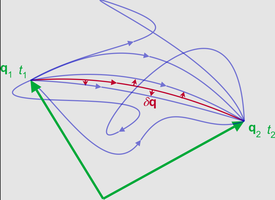
A chart showing the lines of several mathematical functions. — The principle of least action indicates which trajectory is the correct one. In this figure, q represents the generalized coordinate.
Maschen/Wikimedia Commons (CC0 1.0)&ZeroWidthSpace;

In calculus, students learn to find the highest and lowest points of a function within a given interval or across its domain. These highest and lowest points are known collectively as the extrema. You find them through curve sketching: you differentiate and set the result equal to zero. In this case, however, the action isn’t a simple function but a specific type of function called a functional—yes, those two little letters make a difference. The action integrates the Lagrangian over time, and the Lagrangian itself consists of time-dependent functions, such as the velocity and position of the object in question. Therefore, you must proceed more carefully to determine the extrema of the action.

One way to do this is through the calculus of variations. The principle is similar to that used for ordinary functions: you tweak the possible trajectories that the system can follow and find out where the action changes the least. In this way, you obtain equations that correspond to the equations of motion of the system being described—for example, the orbits of planets.

Noether’s Trick: Every Symmetry Brings a Conserved Quantity

After this foray into theoretical physics and calculus, you’re probably wondering what all of this has to do with Noether’s theorem. In fact, the Lagrangian allows us to determine the continuous symmetries of a given system.

If we apply a symmetry transformation (such as a shift in the x coordinates) to the variables of the Lagrangian L without changing anything, then we have found a symmetry. For example, if we want to describe two spheres moving toward each other along the x axis and colliding, the Lagrangian depends solely on their distance: s1 − s2 = q, where q is the generalized coordinate, s1 the position of sphere one and s2 the position of sphere 2. If we shift the positions of both spheres by the same distance α, the Lagrangian remains the same because (s1 + α) − (s2 + α) = q. Therefore the system is symmetric with respect to translation.

Noether investigated how any Lagrangian changes when a variable (such as time or position) is varied by a parameter α. This change in Lis best analyzed by taking the derivative of the Lagrangian with respect to α. If the change as a result of α represents a symmetry transformation, L will not change—consequently, the derivative is zero.

By utilizing some properties of the Lagrangian and performing a few transformations, the derivative of L with respect to α, or (∂L/∂α), becomes the derivative of a new expression Q with respect to time (dQ/dt). And this is also zero—that is, the new expression Q does not change over time and is therefore a conserved quantity! Thus, Noether’s theorem provides a conserved quantity for every symmetry and even gives a formula for calculating this quantity.

This article originally appeared in Spektrum der Wissenschaft and was reproduced with permission. It was translated from the original German version with the assistance of artificial intelligence and reviewed by our editors.

It’s Time to Stand Up for Science

If you enjoyed this article, I’d like to ask for your support. Scientific American has served as an advocate for science and industry for 180 years, and right now may be the most critical moment in that two-century history.

I’ve been a Scientific American subscriber since I was 12 years old, and it helped shape the way I look at the world. SciAm always educates and delights me, and inspires a sense of awe for our vast, beautiful universe. I hope it does that for you, too.

If you subscribe to Scientific American, you help ensure that our coverage is centered on meaningful research and discovery; that we have the resources to report on the decisions that threaten labs across the U.S.; and that we support both budding and working scientists at a time when the value of science itself too often goes unrecognized.

In return, you get essential news, captivating podcasts, brilliant infographics, can't-miss newsletters, must-watch videos, challenging games, and the science world's best writing and reporting. You can even gift someone a subscription.

There has never been a more important time for us to stand up and show why science matters. I hope you’ll support us in that mission.

Thank you,

David M. Ewalt, Editor in Chief, Scientific American

AI finds hidden ECG signal that predicts sudden cardiac death risk

Sudden cardiac death kills more than 300,000 people in the U.S. each year, even though implantable defibrillators have been able to stop many lethal arrhythmias for decades. The main issue today isn’t the device that stops a cardiac arrest; it is figuring out who needs one. In a new Nature study, a team led by Ziad Obermeyer, an associate professor at the University of California, Berkeley, trained a neural network to answer that question from a 10-second electrocardiogram. Then they trained a second neural network to reveal what the first was keying on.

The two-model setup points to a larger ambition for AI in medicine: getting a machine to surface a fresh clue that human experts can then see and check for themselves. Obermeyer’s team used the first network to predict risk and the second to translate that prediction into a visible feature on an ordinary ECG, one a cardiologist could learn to spot.

To decide who should get a defibrillator, cardiologists currently lean on an ultrasound measurement of how much blood the left ventricle pumps with each beat—a measure known as left ventricular ejection fraction, or LVEF. Obermeyer points out that it is far from perfect. “A lot of people who suddenly die of cardiac arrest either never had the ultrasound before or they had it and the results were normal,” he says. At the same time, most defibrillators implanted on the strength of that test never end up firing. “Often a person who looked high risk turned out not to be so high risk after all,” Obermeyer says. To get around the problem, his team went looking for a better risk marker.

On supporting science journalism

Electrocardiograms, or ECGs, measure the heart’s electrical activity and are cheap and nearly universal by comparison. Yet despite decades of studying ECG waveforms, cardiologists had never found a pattern that reliably flagged a high risk of cardiac arrest. His team turned to deep learning to find the pattern that human inspection had missed. The algorithm the team picked was a 64-layer residual neural network, or ResNet. “It’s kind of a workhorse model everyone uses. There’s nothing interesting about it,” Obermeyer says. “What is interesting is the data it’s learned from.”

To feed the network, Obermeyer’s group assembled one of the first population-scale datasets of its kind, with more than 440,000 ECGs from roughly 180,000 patients in Sweden, matched to national death certificates. Trained on the Swedish data, the otherwise generic ResNet flagged a high-risk group amounting to about 2.2 percent of patients. The signal held up when the team tested the model on separate datasets from the U.S. and Taiwan, suggesting this wasn’t a quirk of Sweden’s population or ECG equipment. Within that small group, the annual rate of sudden cardiac death reached 7 percent—well above the 4.6 percent rate among patients flagged by the standard ultrasound test. What’s more, more than 86 percent of the patients the algorithm singled out were not flagged by the traditional LVEF marker. By the traditional measure, many patients like these would have been sent home without a defibrillator.

“After we established this thing is working, we wanted to understand what this model is seeing in the ECG waveforms of high-risk people,” Obermeyer says. Standard AI interpretability tools like saliency maps can highlight which parts of a waveform a neural net weighted most heavily, but they stop there. A human cardiologist who spots something unusual on an ECG trace can sketch the anomalous wave. A neural network, by default, cannot. So, Obermeyer and his colleagues built a generative AI model to do just that. “Its job was to produce ECG waveforms that looked high-risk to the first model,” Obermeyer says.

Paired with the original network and guided by its risk score, the generative model reworked a real low-risk patient’s ECG step by step, morphing it smoothly into a high-risk version of the same trace. Many of the features the model keyed on were already familiar to cardiologists.

One feature, though, had never been described in the medical literature: a subtle slurring in one ECG lead called aVL, suggesting that the heart’s electrical signal was fragmenting as it moved through muscle.

Changxin Lai, a biomedical engineer at Johns Hopkins University who wrote an accompanying analysis in Natureand was not involved in the study, says this is why the work stands out. “The ECG has been around for more than 100 years, and this kind of data has been carefully evaluated by generations of cardiologists,” he says. “We extracted new knowledge from an artificial intelligence model.”

For some of the high-risk patients, the team also had cardiac magnetic resonance imaging, or MRI, scans. Those scans showed subtle, diffuse fibrosis, scarring associated with arrhythmias that can interfere with the heart’s electrical signals in a way that fits the synthetic waveforms the generative model produced. Obermeyer cautions that the fibrosis link is preliminary and has yet to be confirmed with biopsies.

The finding, while intriguing, is not ready to guide treatment. “This is an important area of research,” says Sumeet S. Chugh, who directs the Center for Cardiac Arrest Prevention at Cedars-Sinai Medical Center and was not involved in the study. “But from a patient care perspective there is much more research to be done before we will be using such findings to… identify candidates for the primary prevention implantable defibrillator,” he adds.

Even so, Obermeyer thinks the approach is worth pursuing. “There are some very fancy imaging techniques like MRI, but these things are not feasible for screening populations because of their expense and inconvenience,” Obermeyer says. ECGs, he argues, sit at the opposite end of the spectrum; they can be recorded nearly anywhere, with an Apple Watch or a simple device that connects to a smartphone. The team acknowledges that the model was trained on medical-grade ECGs and performs slightly worse on the lower-quality signals from consumer devices, though by a margin they describe as minor.

“I wouldn’t suggest going out and getting a defibrillator implanted just because we say your ECG is high risk,” Obermeyer says. “What’s nice about this is you don’t have to believe the AI at all. You can just use it to target additional testing like doing traditional risk markers.”